Extracting and Cleaning Bibliometric Data with R (1)
Exploring Scopus

Table of Contents
After the roadmap for learning to programme in R where I listed useful tutorials and packages, I propose here to get to the heart of the matter and to learn how to extract and clean bibliometric data. This tutorial keeps in mind the issues that historians of economics can encounter, but I hope it could be also useful for other social scientists.
It is not easy to navigate between the different existing bibliometric database (Web of Science, Scopus, Dimensions, Jstor, Econlit, RePEc…), and to know which information they gather and how much data we can extract. I will thus bring here a series of tutorials on how to find and extract such data (if possible, by doing it via R scripts), but also on how to clean them. Indeed, depending on the database one uses, the data are in different formats, and one often has to do some cleaning (notably for the bibliographic references cited by the corpus one has extracted). In this tutorial, we will focus on Scopus data for which you will need an institutional access. The next post focuses on Dimensions data and the one after will deal with Constellate application of JSTOR. Both Dimensions and Constellate are accessible without institutional access.
At the end of this tutorial, you will know how to get the data needed for building bibliographic networks and I will give an example of a co-citation network using the biblionetwork package (Goutsmedt, Claveau, and Truc 2021). What you only need in this tutorial is a basic understanding of some functions of Tidyverse packages (Wickham 2021; Wickham et al. 2019)—mainly dplyr and stringr—as well as a (less) basic understanding of “regex” (Regular Expressions).1 At some points I dig into more complicated and tortuous methods when using Elsevier/Scopus APIs with rscopus or cleaning references with the machine learning software anystyle using the command line. This will be explained in separated sections that beginners can skip.
Let’s first load all the packages we need and set the path to the directory where I put the data extracted from Scopus:
# packages
package_list <- c(
  "here", # use for paths creation
  "tidyverse",
  "bib2df", # for cleaning .bib data
  "janitor", # useful functions for cleaning imported data
  "rscopus", # using Scopus API
  "biblionetwork", # creating edges
  "tidygraph", # for creating networks
  "ggraph" # plotting networks
)
for (p in package_list) {
  if (p %in% installed.packages() == FALSE) {
    install.packages(p, dependencies = TRUE)
  }
  library(p, character.only = TRUE)
}

github_list <- c(
  "agoutsmedt/networkflow", # manipulating network
  "ParkerICI/vite" # needed for the spatialisation of the network
)
for (p in github_list) {
  if (gsub(".*/", "", p) %in% installed.packages() == FALSE) {
    devtools::install_github(p)
  }
  library(gsub(".*/", "", p), character.only = TRUE)
}

# paths
data_path <- here(path.expand("~"),
                  "data",
                  "tuto_biblio_dsge")
scopus_path <- here(data_path,
                    "scopus")
Extracting data from Scopus
Using Scopus website
I focus here on a not so much historical subject because a very recent one: the Dynamic Stochastic General Equilibrium (DSGE) models. This type of models has emerged in the late 1990s and has become standard in academic publications as well as in policymaking institutions, notably in central banks.2
If you don’t have one, you will need to create an account on Scopus using your institutional email address. Once you are on the “Documents” query page, you can search for “DSGE” or “Dynamic Stochastic General Equilibrium” in documents titles, abstracts and keywords (see Figure 1). On January 2022, I got 2633 results. You can select “All” the documents and then click on the down arrow on the righ of “CSV export” (see Figure 2). You then have to choose all the information you want to download in a .csv. What we need is to cross the “Include References” box as we need it for the bibliographic co-citation later (see Figure 3).3
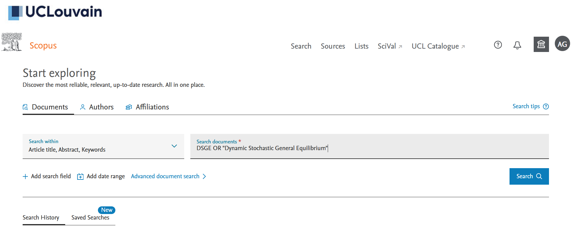
Figure 1: Scopus search page
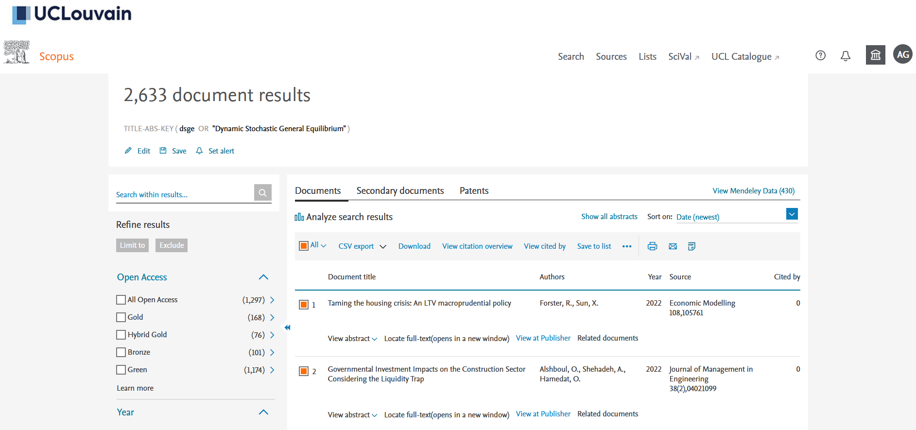
Figure 2: Scopus results page
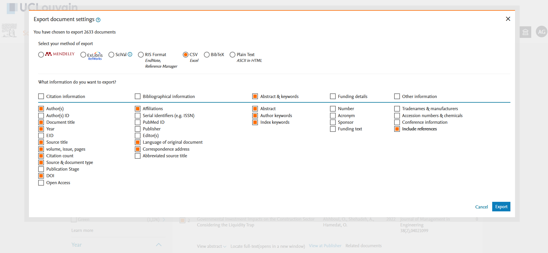
Figure 3: Choosing the information to export in a CSV
The .csv you have exported gathers metadata on authors, title, journal, abstract, keywords, affiliations and references on documents (mainly articles, but also conference papers, book chapters, and reviews) mentioning DSGE in their title, abstract or keywords. There are two limits at this method for extracting data:
- the quantity of data you can export is limited to 2000, which is not much;
- part of the metadata are relatively raw, like affiliations and references, what involves some cleaning.
I will show you how to clean these raw data in the next section. But the following sub-section explains you how to use Scopus APIs directly in R, to query more easily for different data and extract more items.
Alternative method: Using Scopus APIs and rscopus
You first need to create an “API Key” on Scopus website (see more info here) associated to your account. Using the APIs allows you to extract larger set of data (see the available APIs and corresponding quotas here).
Let’s use Rscopus and set the API key:
api_key <- "your_api_key"
set_api_key(api_key)
Most of the time (and it was the case for me) your institutional access is linked to an IP address and you are not able to use the APIs if you are not connected to your institution internet network. If you want to work remotely, you need to ask for a “token-based” authentification ad ask for an “Institutional Token” or “Insttoken” (see explanations here). You just have to write to Elsevier to explain which kind of research you are doing and ask them for an “insttoken”. That is also a good occasion, if necessary, to ask them for higher quotas.
Let’s set the institutional token:
insttoken <- "your_institutional_token"
insttoken <- inst_token_header(insttoken)
We first run the query using “Scopus Search API” via rscopus. That is the API corresponding to the search we have done above on Scopus website. We can now extract as much as 20000 items directly per week. We get raw data with a lot of information in it (the data but also information on the query, etc.). Using rscopus gen_entries_to_df function, we convert these raw data in data.frames.
dsge_query <- rscopus::scopus_search("TITLE-ABS-KEY(DSGE) OR TITLE-ABS-KEY(\"Dynamic Stochastic General Equilibrium\")",
                                     view = "COMPLETE",
                                     headers = insttoken)
dsge_data_raw <- gen_entries_to_df(dsge_query$entries)
We can finally separate the different data.frames. We get three tables with different types of information:
- A table with all the articles and their metadata;
- A table with the list of all authors of the articles;
- A table with the list of affiliations.
dsge_papers <- dsge_data_raw$df
dsge_affiliations <- dsge_data_raw$affiliation
dsge_authors <- dsge_data_raw$author
Now that we have the articles, we have to extract the references using scopus “Abstract Retrieval API”. We use articles internal identifier to find references. But we cannot query references with multiple identifiers, so we need to make a loop to extract references one by one. We create a list where we put the references for each articles (we have as many data.frames as articles in our list) and we bind the data.frames together, associating each of them to the identifier of the corresponding citing article.4
[Modification from November 16, 2023, following a comment by Olivier:] Another issue with extracting references is that you cannot extract more than 40 references per article. If an article has more than 40 references in its bibliography, you need to make a loop in order to collect all the references.
citing_articles <- dsge_papers$`dc:identifier` # extracting the IDs of our articles on dsge
citation_list <- list()

for(i in 1:length(citing_articles)){
  citations_query <- abstract_retrieval(citing_articles[i],
                                        identifier = "scopus_id",
                                        view = "REF",
                                        headers = insttoken)
  if(!is.null(citations_query$content$`abstracts-retrieval-response`)){ # Checking if the article has some references before collecting them

    nb_ref <- as.numeric(citations_query$content$`abstracts-retrieval-response`$references$`@total-references`)
    citations <- gen_entries_to_df(citations_query$content$`abstracts-retrieval-response`$references$reference)$df

    if(nb_ref > 40){ # The loop to collect all the references
      nb_query_left_to_do <- floor((nb_ref) / 40)
      cat("Number of requests left to do :", nb_query_left_to_do, "\n")
      for (j in 1:nb_query_left_to_do){
        cat("Request n°", j , "\n")
        citations_query <- abstract_retrieval(citing_articles[i],
                                              identifier = "scopus_id",
                                              view = "REF",
                                              startref = 40*j+1,
                                              headers = insttoken)
        citations_sup <- gen_entries_to_df(citations_query$content$`abstracts-retrieval-response`$references$reference)$df
        citations <- bind_rows(citations, citations_sup)
      }
    }

    citations <- citations %>%
      as_tibble(.name_repair = "unique") %>%
      select_if(~!all(is.na(.)))

    citation_list[[citing_articles[i]]] <- citations
  }
}

dsge_references <- bind_rows(citation_list, .id = "citing_art")
Once you have these four data.frames (articles metadata, authors, affiliations and references), you can proceed to the bibliometric analysis. The only difficulty now is to navigate between the numerous columns of each data.frame and to understand what the different information are. To link the articles metadata data.frame with the reference one, you can use the scopus identifier that we have put in the reference table (in the column citing_art). If you want to join the articles metadata data.frame with the authors and affiliations ones, you have to use the entry_number column that exists in the three data.frames. This number is created by Scopus after your query, meaning that articles, affiliations and authors are not linked by a permanent identifier. Consequently, the identifiers will be regenerated and thus different if you change your query.
In addition to saving you the laborious task of cleaning references and affiliations, when you use the APIs, the references already have an identifier, given by Scopus. It means that if two articles cite the same reference, you will know it because this reference will have a common identifier in the citations of both the first and second article. Below, when manipulating the data extracted from Scopus website, we will need to find which citations are corresponding to the same reference ourselves.5
If you are not to afraid by Scopus categories and language, or by querying a website through an R script, that is perhaps the quickest method to get data (and that is a method that allows you to get more data, with more complicated queries). However, in the next section, I show you how to clean the data extracted from the Scopus website above.
Cleaning Scopus data
So let’s come back to the data we have downloaded on Scopus website:
#' # Cleaning scopus data from website search
#'

scopus_search_1 <- read_csv(here(scopus_path, "scopus_search_1998-2013.csv"))
scopus_search_2 <- read_csv(here(scopus_path, "scopus_search_2014-2021.csv"))
scopus_search <- rbind(scopus_search_1, scopus_search_2) %>%
  mutate(citing_id = paste0("A", 1:n())) %>% # We create a unique ID for each doc of our corpus
  clean_names() # janitor function to clean column names

scopus_search
## # A tibble: 2,608 × 23
##    authors      title  year source_title volume issue art_no page_start page_end
##    <chr>        <chr> <dbl> <chr>        <chr>  <chr> <chr>  <chr>      <chr>
##  1 Ha J., So I. Infl…  2013 Global Econ… 42     4     <NA>   396        424
##  2 Botero J., … Exog…  2013 Revista de … 16     1     <NA>   1          24
##  3 Kirsanova T… Comm…  2013 Internation… 9      4     <NA>   99         151
##  4 Ashimov A.A… Para…  2013 Economic De… <NA>   <NA>  <NA>   95         188
##  5 Khan A., Th… Cred…  2013 Journal of … 121    6     <NA>   1055       1107
##  6 Jeřábek T.,… Pred…  2013 Acta Univer… 61     7     <NA>   2229       2238
##  7 Hu X., Xu B… Infl…  2013 Journal of … 5      12    <NA>   636        641
##  8 Cha H.       Taki…  2013 Internation… 7      2     <NA>   280        296
##  9 da Silva M.… The …  2013 North Ameri… 26     <NA>  <NA>   266        281
## 10 Sandri D., … Fina…  2013 Journal of … 45     SUPP… <NA>   59         86
## # ℹ 2,598 more rows
## # ℹ 14 more variables: page_count <dbl>, cited_by <dbl>, doi <chr>,
## #   affiliations <chr>, authors_with_affiliations <chr>, abstract <chr>,
## #   author_keywords <chr>, index_keywords <chr>, references <chr>,
## #   correspondence_address <chr>, language_of_original_document <chr>,
## #   document_type <chr>, source <chr>, citing_id <chr>
There are several things to clean:
- We have several
authorsper document. For some analysis, for instance co-authorship networks, it is better to have an “author table” which associates each author to a list of papers; - We have several
affiliationsper article as well as severalauthors_with_affiliations. It allows us to connect authors with their affiliations, but here again we need to separate it in as many lines as authors (if I am not mistaken, it seems there is only one affiliation per author in this set of data); references;- Possibly to separate
author_keywordsandindex_keywordsif you want to use it.
In what follows, we clean scopus_search in order to produce 3 additional data.frames:
- one
data.framewhich associates each article to a list of authors and their corresponding affiliation (see below); - one data.frame which associate each article to the list of references it cites (one article has as many lines as the number of cited references): this is a “direct citation” table (see here);
- a list of all the references cited, which implies to find which references are the same in the direct citation table (see this sub-section)
Extracting affiliations and authors
We have two columns for affiliations:
- one column
affiliationswith affiliations alone; - one column,
authors_with_affiliationswith both authors and affiliations.
affiliations_raw <- scopus_search %>%
  select(citing_id, authors, affiliations, authors_with_affiliations)

knitr::kable(head(affiliations_raw, n = 2))
| citing_id | authors | affiliations | authors_with_affiliations |
|---|---|---|---|
| A1 | Ha J., So I. | Department of Economics, Cornell University, Ithaca, NY, United States; Department of Economics, University of Washington, Seattle, WA, United States | Ha, J., Department of Economics, Cornell University, Ithaca, NY, United States; So, I., Department of Economics, University of Washington, Seattle, WA, United States |
| A2 | Botero J., Franco H., Hurtado Á., Mesa M. | Departamento de Economía, Universidad EAFIT, Medellín, Colombia; EAFIT University, Colombia | Botero, J., Departamento de Economía, Universidad EAFIT, Medellín, Colombia; Franco, H., Departamento de Economía, Universidad EAFIT, Medellín, Colombia; Hurtado, Á., Departamento de Economía, Universidad EAFIT, Medellín, Colombia; Mesa, M., EAFIT University, Colombia |
For a more secure cleaning, we opt for the second column, as it allows us to associate the author with his/her own affiliation as described in the column authors_with_affiliations. The strategy here is to separate each author from the authors column, then to separate the different authors and affiliations in the authors_with_affiliations column. Finally, we keep only the lines where the author from authors_with_affiliations is the same as in authors
scopus_affiliations <- affiliations_raw %>%
  separate_rows(authors, sep = ", ") %>%
  separate_rows(contains("with"), sep = "; ") %>%
  mutate(authors_from_affiliation = str_extract(authors_with_affiliations,
                                                "^(.+?)\\.(?=,)"),
         authors_from_affiliation = str_remove(authors_from_affiliation, ","),
         affiliations = str_remove(authors_with_affiliations, "^(.+?)\\., "),
         country = str_remove(affiliations, ".*, ")) %>% # Country is after the last comma
  filter(authors == authors_from_affiliation) %>%
  select(citing_id, authors, affiliations, country)


knitr::kable(head(scopus_affiliations))
| citing_id | authors | affiliations | country |
|---|---|---|---|
| A1 | Ha J. | Department of Economics, Cornell University, Ithaca, NY, United States | United States |
| A1 | So I. | Department of Economics, University of Washington, Seattle, WA, United States | United States |
| A2 | Botero J. | Departamento de Economía, Universidad EAFIT, Medellín, Colombia | Colombia |
| A2 | Franco H. | Departamento de Economía, Universidad EAFIT, Medellín, Colombia | Colombia |
| A2 | Hurtado Á. | Departamento de Economía, Universidad EAFIT, Medellín, Colombia | Colombia |
| A2 | Mesa M. | EAFIT University, Colombia | Colombia |
Clean references
Let’s first extract the references column while keeping the identifier of the citing article. We put each reference cited by an article on a separated line, using the fact that the references are separated by a semi-colon. We create an identifier for each reference.
#' ## Extracting and cleaning references
references_extract <- scopus_search %>%
  filter(! is.na(references)) %>%
  select(citing_id, references) %>%
  separate_rows(references, sep = "; ") %>%
  mutate(id_ref = 1:n()) %>%
  as_tibble

knitr::kable(head(references_extract))
| citing_id | references | id_ref |
|---|---|---|
| A1 | Bernanke, B., Gertler, M., Gilchrist, S., Financial accelerator in a quantitative business cycle framework, NBER Working Paper No. W6455 (1998), NBER | 1 |
| A1 | Calvo, G., Staggered prices in a utility maximizing framework (1983) Journal of Monetary Economics, 12, pp. 383-398 | 2 |
| A1 | Christensen, I., Dib, A., Monetary policy in an estimated DSGE model with a financial accelerator (2005) Computing in Economics and Finance, p. 314 | 3 |
| A1 | Dixit, A., Stiglitz, J., Monopolistic competition and optimum product diversity (1977) American Economic Review, 67 (3), pp. 297-308 | 4 |
| A1 | Gerali, A., Neri, S., Sessa, L., Signoretti, F., Credit and banking in a DSGE model (2010), 42 (6), pp. 107-141. , Working paper, Banka D’Italia, Rome | 5 |
| A1 | Goodfriend, M., McCallum, B., Banking and interest rates in monetary policy analysis: A quantitative exploration (2007), NBER Working Paper Series No. 13207, NBER | 6 |
We now have one reference per line and complications begin. We need to find ways to extract the different pieces of information for each reference: authors, year, pages, volume & issue information, journal, title, etc… Here are some regex that will match some of these information.
extract_authors <- ".*[:upper:][:alpha:]+( Jr(.)?)?, ([A-Z]\\.[ -]?)?([A-Z]\\.[ -]?)?([A-Z]\\.)?[A-Z]\\."
extract_year_brackets <- "(?<=\\()\\d{4}(?=\\))"
extract_pages <- "(?<= (p)?p\\. )([A-Z])?\\d+(-([A-Z])?\\d+)?"
extract_volume_and_number <- "(?<=( |^)?)\\d+ \\(\\d+(-\\d+)?\\)"
We can now extract authors and year. We create a new column, remaining_ref which keeps the information from the references column but we remove the authors from it. For easier cleaning, we separate references depending on the position of the year of publication in the reference. We use the variable is_article to determinate where the year is and thus if the title is before the year or not.
cleaning_references <- references_extract %>%
  mutate(authors = str_extract(references, paste0(extract_authors, "(?=, )")),
         remaining_ref = str_remove(references, paste0(extract_authors, ", ")), # cleaning from authors
         is_article = ! str_detect(remaining_ref, "^\\([:digit:]{4}"),
         year = str_extract(references, extract_year_brackets) %>% as.integer)
I cannot detail all the regex below but the goal is to extract as many relevant metadata as possible, first for references with the year of publication after the title (is_article == TRUE), which are most of the time journal articles.
This code has been written in January 2022 and I will try to improve it later, notably because this use of the
is_articlevariable makes the code unecessarily longer.
cleaning_articles <- cleaning_references %>%
  filter(is_article == TRUE) %>%
  mutate(title = str_extract(remaining_ref, ".*(?=\\(\\d{4})"), # pre date extraction
         journal_to_clean = str_extract(remaining_ref, "(?<=\\d{4}\\)).*"), # post date extraction
         journal_to_clean = str_remove(journal_to_clean, "^,") %>% str_trim("both"), # cleaning a bit the journal info column
         pages = str_extract(journal_to_clean, extract_pages), # extracting pages
         volume_and_number = str_extract(journal_to_clean, extract_volume_and_number), # extracting standard volument and number: X (X)
         journal_to_clean = str_remove(journal_to_clean, " (p)?p\\. ([A-Z])?\\d+(-([A-Z])?\\d+)?"), # clean from extracted pages
         journal_to_clean = str_remove(journal_to_clean, "( |^)?\\d+ \\(\\d+(-\\d+)?\\)"), # clean from extracted volume and number
         volume_and_number = ifelse(is.na(volume_and_number), str_extract(journal_to_clean, "(?<= )([A-Z])?\\d+(-\\d+)?"), volume_and_number), # extract remaining numbers
         journal_to_clean = str_remove(journal_to_clean, " ([A-Z])?\\d+(-\\d+)?"), # clean from remaining numbers
         journal = str_remove_all(journal_to_clean, "^[:punct:]+( )?[:punct:]+( )?|(?<=,( )?)[:punct:]+( )?([:punct:])?|[:punct:]( )?[:punct:]+( )?$"), # extract journal info by removing inappropriate punctuations
         first_page = str_extract(pages, "\\d+"),
         volume = str_extract(volume_and_number, "\\d+"),
         issue = str_extract(volume_and_number, "(?<=\\()\\d+(?=\\))"),
         publisher = ifelse(is.na(first_page) & is.na(volume) & is.na(issue) & ! str_detect(journal, "(W|w)orking (P|p)?aper"), journal, NA),
         book_title = ifelse(str_detect(journal, " (E|e)d(s)?\\.| (E|e)dite(d|urs)? "), journal, NA), # Incollection article: Title of the book here
         book_title = str_extract(book_title, "[A-z ]+(?=,)"), # keeping only the title of the book
         publisher = ifelse(!is.na(book_title), NA, publisher), # if we have an incollection article, that's not a book, so no publisher
         journal = ifelse(!is.na(book_title) | ! is.na(publisher), NA, journal), # removing journal as what we have is a book
         publisher = ifelse(is.na(publisher) & str_detect(journal, "(W|w)orking (P|p)?aper"), journal, publisher), # adding working paper publisher information in publisher column
         journal = ifelse(str_detect(journal, "(W|w)orking (P|p)?aper"), "Working Paper", journal))

cleaned_articles <- cleaning_articles %>%
  select(citing_id, id_ref, authors, year, title, journal, volume, issue, pages, first_page, book_title, publisher, references)
We do the same now with the remaining references that are less numerous but that are also less easy to clean, due to the fact that the title is not clearly separated from other information (journal or publisher).
cleaning_non_articles <- cleaning_references %>%
  filter(is_article == FALSE) %>%
  mutate(remaining_ref = str_remove(remaining_ref, "\\(\\d{4}\\)(,)? "),
         title = str_extract(remaining_ref, ".*(?=, ,)"),
         pages = str_extract(remaining_ref, "(?<= (p)?p\\. )([A-Z])?\\d+(-([A-Z])?\\d+)?"), # extracting pages
         volume_and_number = str_extract(remaining_ref, "(?<=( |^)?)\\d+ \\(\\d+(-\\d+)?\\)"), # extracting standard volument and number: X (X)
         remaining_ref = str_remove(remaining_ref, " (p)?p\\. ([A-Z])?\\d+(-([A-Z])?\\d+)?"), # clean from extracted pages
         remaining_ref = str_remove_all(remaining_ref, ".*, ,"), # clean dates and already extracted titles
         remaining_ref = str_remove(remaining_ref, "( |^)?\\d+ \\(\\d+(-\\d+)?\\)"), # clean from extracted volume and number
         volume_and_number = ifelse(is.na(volume_and_number), str_extract(remaining_ref, "(?<= )([A-Z])?\\d+(-\\d+)?"), volume_and_number), # extract remaining numbers
         remaining_ref = str_remove(remaining_ref, " ([A-Z])?\\d+(-\\d+)?"), # clean from remaining numbers
         journal = ifelse(str_detect(remaining_ref, "(W|w)orking (P|p)aper"), "Working Paper", NA),
         journal = ifelse(str_detect(remaining_ref, "(M|m)anuscript"), "Manuscript", journal),
         journal = ifelse(str_detect(remaining_ref, "(M|m)imeo"), "Mimeo", journal),
         publisher = ifelse(is.na(journal), remaining_ref, NA) %>% str_trim("both"),
         first_page = str_extract(pages, "\\d+"),
         volume = str_extract(volume_and_number, "\\d+"),
         issue = str_extract(volume_and_number, "(?<=\\()\\d+(?=\\))"),
         book_title = NA) # to be symetric with "cleaned_articles"

cleaned_non_articles <- cleaning_non_articles %>%
  select(citing_id, id_ref, authors, year, title, journal, volume, issue, pages, first_page, book_title, publisher, references)
We merge the two data.frames and:
- we normalize and clean authors’ name to facilitate matching of references later;
- we extract useful information like DOI and PII.
# merging the two files.
cleaned_ref <- rbind(cleaned_articles, cleaned_non_articles)

#' Now we have all the references, we can do a bit of cleaning on the authors name,
#' and extract useful information, like DOI, for matching later.

cleaned_ref <- cleaned_ref %>%
  mutate(authors = str_remove(authors, " Jr\\."), # standardising authors name to favour matching later
         authors = str_remove(authors, "^\\(\\d{4}\\)(\\.)?( )?"),
         authors = str_remove(authors, "^, "),
         authors = ifelse(is.na(authors), str_extract(references, ".*[:upper:]\\.(?= \\d{4})"), authors), # specific case
         journal = str_remove(journal, "[:punct:]$"), # remove unnecessary punctuations at the end
         doi = str_extract(references, "(?<=DOI(:)? ).*|(?<=\\/doi\\.org\\/).*"),
         pii = str_extract(doi, "(?<=PII ).*"),
         doi = str_remove(doi, ",.*"), # cleaning doi
         pii = str_remove(pii, ",.*"), # cleaning pii
  )

knitr::kable(head(cleaned_ref, n = 3))
| citing_id | id_ref | authors | year | title | journal | volume | issue | pages | first_page | book_title | publisher | references | doi | pii |
|---|---|---|---|---|---|---|---|---|---|---|---|---|---|---|
| A1 | 1 | Bernanke, B., Gertler, M., Gilchrist, S. | 1998 | Financial accelerator in a quantitative business cycle framework, NBER Working Paper No. W6455 | NA | NA | NA | NA | NA | NA | NBER | Bernanke, B., Gertler, M., Gilchrist, S., Financial accelerator in a quantitative business cycle framework, NBER Working Paper No. W6455 (1998), NBER | NA | NA |
| A1 | 2 | Calvo, G. | 1983 | Staggered prices in a utility maximizing framework | Journal of Monetary Economics | 12 | NA | 383-398 | 383 | NA | NA | Calvo, G., Staggered prices in a utility maximizing framework (1983) Journal of Monetary Economics, 12, pp. 383-398 | NA | NA |
| A1 | 3 | Christensen, I., Dib, A. | 2005 | Monetary policy in an estimated DSGE model with a financial accelerator | Computing in Economics and Finance | NA | NA | 314 | 314 | NA | NA | Christensen, I., Dib, A., Monetary policy in an estimated DSGE model with a financial accelerator (2005) Computing in Economics and Finance, p. 314 | NA | NA |
Practically speaking, if you are targetting a serious quantitative work, more cleaning would be needed to remove small errors. As often in this kind of automatised cleaning, 95% of cleaning can be done with few lines of code, and the rest involves many more work. I do not go further here as this is just a tutorial.
Matching references
What we need to do now is to find which references are the same, to give them a unique ID. The trade-off is to match as many true positive as possible (references that are the same) while avoiding to match false positive, that is references that have some information in common, but that actually are not the same references. For instance, matching only by the authors’ names and the year of publication is too broad, as these authors can have published several articles during the same year. Here are several ways to identify a common reference that bear very few risks of matching together different references:
- same first author surname or authors, year, volume and page (this is the most secure ones): let’s call them
fayvp&ayvp; - same journal, volume, issue and first page:
jvip; - same author, year and title:
ayt; - same title, year and first page:
typ; - same Doi or PII.6
We extract first author surname to favour matching as there are more possibilities of small differences for several authors that would prevent us to match similar references.7
cleaned_ref <- cleaned_ref %>%
  mutate(first_author = str_extract(authors, "^[[:alpha:]+[']?[ -]?]+, ([A-Z]\\.[ -]?)?([A-Z]\\.[ -]?)?([A-Z]\\.)?[A-Z]\\.(?=(,|$))"),
         first_author_surname = str_extract(first_author, ".*(?=,)"),
         across(.cols = c("authors", "first_author", "journal", "title"), ~toupper(.)))
For each type of matching, we are giving a new id to the matched references, by giving the id_ref of the first references matched. At the end, we compare all the new id created with all the matching methods, and we take the smaller id.
matching_ref <- function(data, id_ref, ..., col_name){
  match <- data %>%
    group_by(...) %>%
    mutate(new_id = min({{id_ref}})) %>%
    drop_na(...) %>%
    ungroup() %>%
    select({{id_ref}}, new_id) %>%
    rename_with(~ paste0(col_name, "_new_id"), .cols = new_id)

  data <- data %>%
    left_join(match)
}

identifying_ref <- cleaned_ref %>%
  matching_ref(id_ref, first_author_surname, year, title, col_name = "fayt") %>%
  matching_ref(id_ref, journal, volume, issue, first_page, col_name = "jvip") %>%
  matching_ref(id_ref, authors, year, volume, first_page, col_name = "ayvp") %>%
  matching_ref(id_ref, first_author_surname, year, volume, first_page, col_name = "fayvp") %>%
  matching_ref(id_ref, title, year, first_page, col_name = "typ") %>%
  matching_ref(id_ref, pii, col_name = "pii") %>%
  matching_ref(id_ref, doi, col_name = "doi")
Now we have our direct citation table connecting the citing articles to the references. We have as many lines as the number of citations by citing articles.
direct_citation <- identifying_ref %>%
  mutate(new_id_ref = select(., ends_with("new_id")) %>%  reduce(pmin, na.rm = TRUE),
         new_id_ref = ifelse(is.na(new_id_ref), id_ref, new_id_ref))  %>%
  relocate(new_id_ref, .after = citing_id) %>%
  select(-id_ref & ! ends_with("new_id"))

knitr::kable(head(filter(direct_citation, new_id_ref == 2), n = 4))
| citing_id | new_id_ref | authors | year | title | journal | volume | issue | pages | first_page | book_title | publisher | references | doi | pii | first_author | first_author_surname |
|---|---|---|---|---|---|---|---|---|---|---|---|---|---|---|---|---|
| A1 | 2 | CALVO, G. | 1983 | STAGGERED PRICES IN A UTILITY MAXIMIZING FRAMEWORK | JOURNAL OF MONETARY ECONOMICS | 12 | NA | 383-398 | 383 | NA | NA | Calvo, G., Staggered prices in a utility maximizing framework (1983) Journal of Monetary Economics, 12, pp. 383-398 | NA | NA | CALVO, G. | Calvo |
| A3 | 2 | CALVO, G. | 1983 | STAGGERED PRICES IN A UTILITY-MAXIMIZING FRAMEWORK | JOURNAL OF MONETARY ECONOMICS | 12 | 3 | 383-398 | 383 | NA | NA | Calvo, G., Staggered Prices in a Utility-Maximizing Framework (1983) Journal of Monetary Economics, 12 (3), pp. 383-398 | NA | NA | CALVO, G. | Calvo |
| A18 | 2 | CALVO, G. | 1983 | STAGGERED PRICES IN A UTILITY MAXIMIZING FRAMEWORK | JOURNAL OF MONETARY ECONOMICS | 12 | NA | 383-398 | 383 | NA | NA | Calvo, G., Staggered prices in a utility maximizing framework (1983) Journal of Monetary Economics, 12, pp. 383-398 | NA | NA | CALVO, G. | Calvo |
| A20 | 2 | CALVO, G.A. | 1983 | STAGGERED PRICES IN A UTILITY-MAXIMIZING FRAMEWORK | JOURNAL OF MONETARY ECONOMICS | 12 | 3 | 383-398 | 383 | NA | NA | Calvo, G.A., Staggered prices in a utility-maximizing framework (1983) Journal of Monetary Economics, 12 (3), pp. 383-398 | NA | NA | CALVO, G.A. | Calvo |
We can extract the list of all the references cited. We have as many lines as references cited by citing articles (i.e. a reference cited multiple times is present only once in the table). As for matched references, we have different information (due to the fact that the references were cited differently depending on the citing articles), we take a line where information seems to be the most complete.
important_info <- c("authors",
                    "year",
                    "title",
                    "journal",
                    "volume",
                    "issue",
                    "pages",
                    "book_title",
                    "publisher")
references <- direct_citation %>%
  mutate(nb_na = rowSums(!is.na(select(., all_of(important_info))))) %>%
  group_by(new_id_ref) %>%
  slice_max(order_by = nb_na, n = 1, with_ties = FALSE) %>%
  select(-citing_id) %>%
  unique

knitr::kable(head(references, n = 4))
| new_id_ref | authors | year | title | journal | volume | issue | pages | first_page | book_title | publisher | references | doi | pii | first_author | first_author_surname | nb_na |
|---|---|---|---|---|---|---|---|---|---|---|---|---|---|---|---|---|
| 1 | BERNANKE, B., GERTLER, M., GILCHRIST, S. | 1998 | FINANCIAL ACCELERATOR IN A QUANTITATIVE BUSINESS CYCLE FRAMEWORK, NBER WORKING PAPER NO. W6455 | NA | NA | NA | NA | NA | NA | NBER | Bernanke, B., Gertler, M., Gilchrist, S., Financial accelerator in a quantitative business cycle framework, NBER Working Paper No. W6455 (1998), NBER | NA | NA | BERNANKE, B. | Bernanke | 4 |
| 2 | CALVO, G. | 1983 | STAGGERED PRICES IN A UTILITY-MAXIMIZING FRAMEWORK | JOURNAL OF MONETARY ECONOMICS | 12 | 3 | 383-398 | 383 | NA | NA | Calvo, G., Staggered Prices in a Utility-Maximizing Framework (1983) Journal of Monetary Economics, 12 (3), pp. 383-398 | NA | NA | CALVO, G. | Calvo | 7 |
| 3 | CHRISTENSEN, I., DIB, A. | 2005 | MONETARY POLICY IN AN ESTIMATED DSGE MODEL WITH A FINANCIAL ACCELERATOR | COMPUTING IN ECONOMICS AND FINANCE | NA | NA | 314 | 314 | NA | NA | Christensen, I., Dib, A., Monetary policy in an estimated DSGE model with a financial accelerator (2005) Computing in Economics and Finance, p. 314 | NA | NA | CHRISTENSEN, I. | Christensen | 5 |
| 4 | DIXIT, A., STIGLITZ, J. | 1977 | MONOPOLISTIC COMPETITION AND OPTIMUM PRODUCT DIVERSITY | AMERICAN ECONOMIC REVIEW | 67 | 3 | 297-308 | 297 | NA | NA | Dixit, A., Stiglitz, J., Monopolistic competition and optimum product diversity (1977) American Economic Review, 67 (3), pp. 297-308 | NA | NA | DIXIT, A. | Dixit | 7 |
From the initial 105313 citations, we get 52577 different references, with 10631 cited at least twice.
We also remove the references column of the initial data.frame as references cited are now gathered in direct_citation.
corpus <- scopus_search %>%
select(-references)
I imagine that after so many steps, you can’t wait to look at these data on DSGE models. But you will have to wait, as the following subsection presents you another method to clean (without cleaning yourself) the references. Or you can go directly to the last section that explores the cleaned data.
Alternative method: anystyle
anystyle is a great references parser relyng on machine learning heuristics. It has an online version where you can put the text for which you want to identify references. However, we will use the command line in order to identify more references than what the online website allows (10 000 while we have 105313 raw references).
Anystyle can be installed as a RubyGem. You thus need to install Ruby (here for Windows) and then install anystyle using the command line: gem install anystyle (see more information here). As you need to use the command line interface, you also need to install anystyle-cli: gem install anystyle-cli.
Some frightened reader: “What, what? wait! Command line you said?”
Oh, yes. And that is a good occasion to refer you to these great tutorials of the great Programming Historian Website: one for the bash command line and one for the Windows Powershell Command Line. And it will be the occasion to use a bit Rstudio Terminal to enter the commands.
Once you have installed anystyle, you need to save all the references (with one reference per line) in a .txt.
ref_text <- paste0(references_extract$references, collapse = "\\\n")
name_file <- "ref_in_text.txt"
write_file(ref_text,
           here(scopus_path,
                name_file))
To create the anystyle command, you need to name the repository where you will send the .bib created by anystyle from your .txt
destination_anystyle <- "anystyle_cleaned"

directory_command <- paste0("cd ", scopus_path)
anystyle_command <- paste0("anystyle -f bib parse ",
                           name_file,
                           " ",
                           destination_anystyle)
To use anystyle, you have to use the command line of the terminal. You first have to set the path where the .txt is (which is here the scopus_path): cd the_path_where_is_the_.txt.
Then you copy and paste the anystyle command in the terminal, which here is:
anystyle -f bib parse ref_in_text.txt anystyle_cleaned. Hopefully it will work and you wil just have to wait for the creation of the .bib (it took something like 10 minutes on my laptop).8
…waiting…
Once we have our .bib, we transform it in a data frame thanks to the bib2df package.
options(encoding = "UTF-8")
bib_ref <- bib2df(here(scopus_path,
                       destination_anystyle,
                       "ref_in_text.bib"))
bib_ref <- bib_ref %>%
  janitor::clean_names() %>%
  select_if(~!all(is.na(.))) %>%  # removing all empty columns
  mutate(id_ref = 1:n()) %>%
  select(-c(translator, citation_number, arxiv, director, source))

knitr::kable(head(bib_ref))
| category | bibtexkey | address | author | booktitle | edition | editor | institution | journal | note | number | pages | publisher | school | series | title | type | volume | date | issue | url | isbn | doi | id_ref |
|---|---|---|---|---|---|---|---|---|---|---|---|---|---|---|---|---|---|---|---|---|---|---|---|
| ARTICLE | bernanke1998a | NA | Bernanke, B. , Gertler, M. , Gilchrist, S. | NA | NA | NA | NA | NBER Working Paper | NA | W6455 | NA | NA | NA | NA | Financial accelerator in a quantitative business cycle framework | NA | 1998 | NA | NA | NA | NA | 1 | |
| ARTICLE | calvo-a | NA | Calvo, G. | NA | NA | NA | NA | Journal of Monetary Economics | NA | NA | 383–398 | NA | NA | NA | Staggered prices in a utility maximizing framework (1983 | NA | 12 | NA | NA | NA | NA | NA | 2 |
| ARTICLE | christensen-a | NA | Christensen, I., Dib, A. | NA | NA | NA | NA | Computing in Economics and Finance | NA | NA | 314 | NA | NA | NA | Monetary policy in an estimated DSGE model with a financial accelerator (2005 | NA | NA | NA | NA | NA | NA | NA | 3 |
| ARTICLE | dixit-a | NA | Dixit, A. , Stiglitz, J. | NA | NA | NA | NA | American Economic Review | NA | 3 | 297–308 | NA | NA | NA | Monopolistic competition and optimum product diversity (1977 | NA | 67 | NA | NA | NA | NA | NA | 4 |
| BOOK | gerali2010a | Banka D’Italia, Rome | Gerali, A. , Neri, S. , Sessa, L. , Signoretti, F. | NA | NA | NA | NA | NA | NA | NA | 107–141 | , Working paper | NA | NA | Credit and banking in a DSGE model | NA | 42 | 2010 | 6 | NA | NA | NA | 5 |
| INCOLLECTION | goodfriend-a | NA | Goodfriend, M., McCallum, B. | NBER Working Paper Series No. 13207, NBER\ | NA | NA | NA | NA | NA | NA | NA | NA | NA | NA | Banking and interest rates in monetary policy analysis: A quantitative exploration (2007 | NA | NA | NA | NA | NA | NA | NA | 6 |
For now, there is one major limitation to this method (which is most likely linked to my lack of mastery of anystyle and ruby): the result is a list of unique references. In other words, anystyle merge together references that are similar. It means that I have to find a way to build a link between the original references data.frame and the data.frame build on the .bib.9
Ideally, you can clean a bit the result. Anystyle is pretty good (and clearly better than I) for identifying the types of references, and thus to extract book title for chapter in books and editors. It is quite efficient to extract authors and titles even if I have seen many mistakes (but relatively easy to clean, as most of the time it is the year that has been put with the title). However, I also saw many mistakes for journals (incomplete name) that are not so easy to correct. If you want to clean your references data as much as possible, perhaps the best thing to do is to mix the coding cleaning approach used above with the anystyle method, and to complete missing information with one or another method.
Exploring the DSGE literature
Now we have our bibliographic data, the first thing we can look at is the most cited references in our corpus.
direct_citation %>%
  add_count(new_id_ref) %>%
  select(new_id_ref, n) %>%
  unique() %>%
  slice_max(n, n = 10) %>%
  left_join(select(references, new_id_ref, references)) %>%
  select(references, n) %>%
  knitr::kable()
| references | n |
|---|---|
| Smets, F., Wouters, R., Shocks and frictions in US business cycles. a Bayesian DSGE approach (2007) American Economic Review, 97 (3), pp. 586-606 | 780 |
| Calvo, G., Staggered Prices in a Utility-Maximizing Framework (1983) Journal of Monetary Economics, 12 (3), pp. 383-398 | 702 |
| Christiano, L.J., Eichenbaum, M., Evans, C.L., Nominal rigidities and the dynamic effects of a shock to monetary policy (2005) Journal of Political Economy, 113 (1), pp. 1-45. , http://ideas.repec.org/a/ucp/jpolec/v113y2005i1p1-45.html | 640 |
| Smets, F., Wouters, R., An Estimated Dynamic Stochastic General Equilibrium Model of the Euro Area (2003) Journal of the European Economic Association, 1 (5), pp. 1123-1175 | 610 |
| Bernanke, B., Gertler, M., Gilchrist, S., The financial accelerator in a quantitative business cycle framework (1999) NBER Working Papers Series, 1 (3), pp. 1341-1393. , Elsevier Science B.V, (chap. 21), Handbook of Macroeconomics | 331 |
| An, S., Schorfheide, F., Bayesian Analysis of DSGE Models (2007) Econometric Reviews, 26 (4), pp. 113-172 | 311 |
| Taylor, J., Discretion versus policy rules in practice (1993) Carnegie-Rochester Conference Series on Public Policy, 39 (0), pp. 195-214 | 269 |
| Iacoviello, M., House prices, borrowing constraints, and monetary policy in the business cycle (2005) American Economic Review, 95 (3), pp. 739-764 | 243 |
| Kydland, F.E., Prescott, E.C., Time to build and aggregate fluctuations (1982) Econometrica, 50 (6), pp. 1345-1370 | 234 |
| Schmitt-Grohe, S., Uribe, M., Closing small open economy models (2003) Journal of International Economics, 61 (1), pp. 163-185 | 228 |
As we have the affiliations, we can try to see which are the top references for economists based in different countries:
direct_citation %>%
  left_join(select(scopus_affiliations, citing_id, country)) %>%
  unique() %>%
  group_by(country) %>%
  mutate(nb_article = n()) %>%
  filter(nb_article > 5000) %>% # we keep only countries with 5000 articles
  add_count(new_id_ref) %>%
  select(new_id_ref, n) %>%
  unique() %>%
  slice_max(n, n = 8) %>%
  left_join(select(references, new_id_ref, references)) %>%
  select(references, n)  %>%
  mutate(label = str_extract(references, ".*\\(\\d{4}\\)") %>%
           str_wrap(30),
         label = tidytext::reorder_within(label, n, country)) %>%
  ggplot(aes(n, label, fill = country)) +
  geom_col(show.legend = FALSE) +
  facet_wrap(~country, ncol = 3, scales = "free") +
  tidytext::scale_y_reordered() +
  labs(x = "Number of citations", y = NULL) +
  theme_classic(base_size = 10)
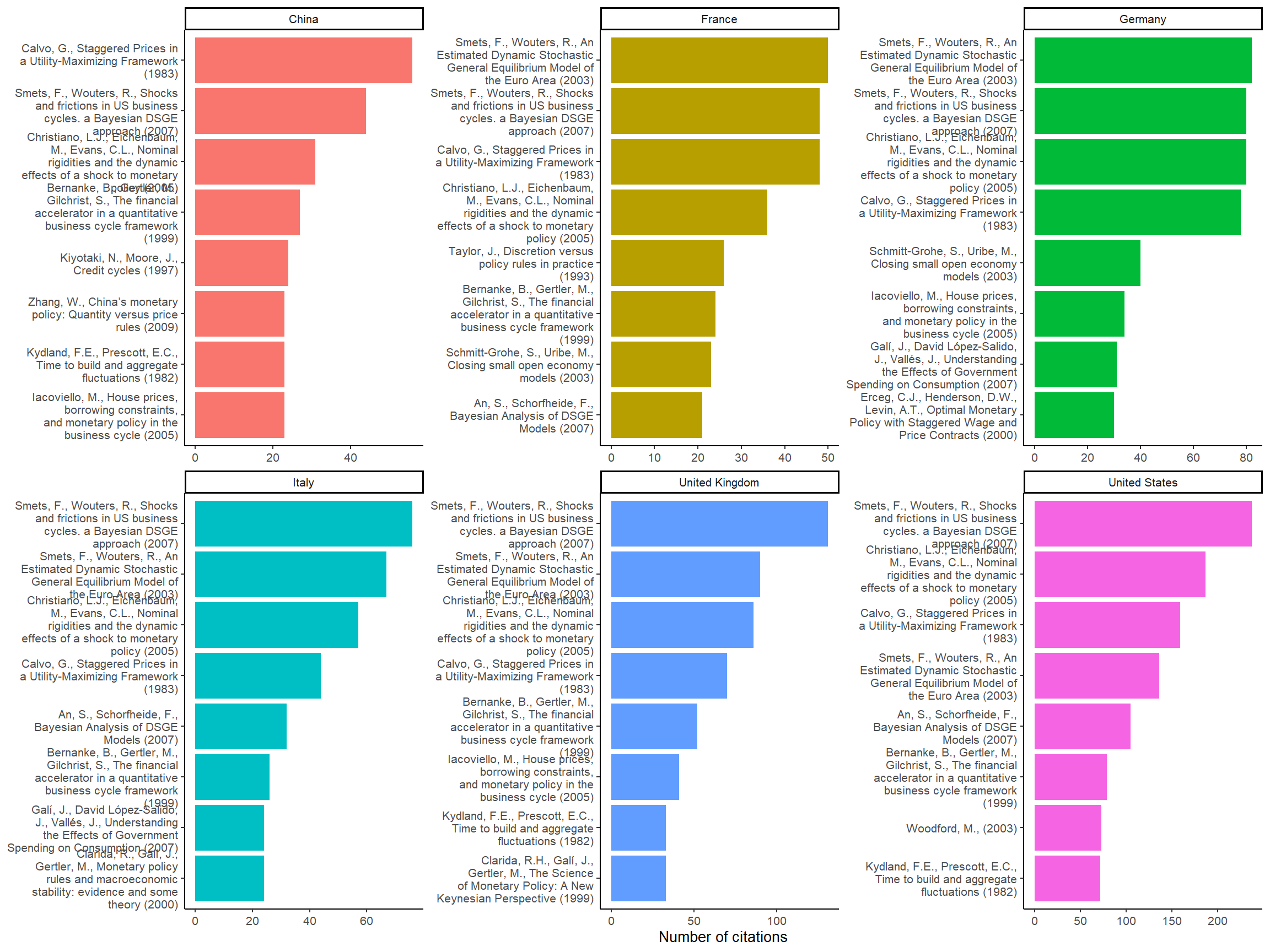
Figure 4: Most cited references per countries
By using affiliations we can observe a regional preference pattern: in European countries, economists tend to cite more Smets and Wouters (2003) (the source of the European Central Bank DSGE model) than Christiano, Eichenbaum, and Evans (2005), while the opposite is true in the United States (Smets and Wouters 2007 is on US data). We can also notice that Kydland and Prescott (1982) is less popular in continental Europe.
Bibliographic co-citation analysis
To conclude this (long) tutorial, we can build a co-citation network: the references we have matched are the nodes of the network, and they are linked together depending on the number of times they are cited together (or in other words, the number of times they are together in a bibliography). We use the biblio_cocitation function of the biblionetwork package. The edge between two nodes is weighted depending of the total number of times each reference has been cited in the whole corpus (see here for more details).
citations <- direct_citation %>%
  add_count(new_id_ref) %>%
  select(new_id_ref, n) %>%
  unique

references_filtered <- references %>%
  left_join(citations) %>%
  filter(n >= 5)

edges <- biblionetwork::biblio_cocitation(filter(direct_citation, new_id_ref %in% references_filtered$new_id_ref),
                                          "citing_id",
                                          "new_id_ref",
                                          weight_threshold = 3)
edges
## Key: <Source>
##          from     to    weight Source Target
##        <char> <char>     <num>  <int>  <int>
##     1:      2      4 0.2354379      2      4
##     2:      2      5 0.1244966      2      5
##     3:      2      6 0.0518193      2      6
##     4:      2      7 0.1623352      2      7
##     5:      2     14 0.1349191      2     14
##    ---
## 42657:  64761  64841 0.4045199  64761  64841
## 42658:  64841  64936 0.3481553  64841  64936
## 42659:  66416  68931 0.7453560  66416  68931
## 42660:  66416  68935 0.5039526  66416  68935
## 42661:  68931  68935 0.6761234  68931  68935
We can then take our corpus and these edges to create a network/graph thanks to tidygraph (Pedersen 2020) and networkflow. I don’t enter in the details here as that is not the purpose of this tutorial and that the different steps are explained on networkflow website.
graph <- tbl_main_component(nodes = references_filtered,
                            edges = edges,
                            directed = FALSE)
graph
## # A tbl_graph: 2836 nodes and 42661 edges
## #
## # An undirected simple graph with 1 component
## #
## # A tibble: 2,836 × 18
##      Id authors      year title journal volume issue pages first_page book_title
##   <int> <chr>       <int> <chr> <chr>   <chr>  <chr> <chr> <chr>      <chr>
## 1     2 CALVO, G.    1983 "STA… JOURNA… 12     3     383-… 383        <NA>
## 2     4 DIXIT, A.,…  1977 "MON… AMERIC… 67     3     297-… 297        <NA>
## 3     5 GERALI, A.…  2010 "CRE… WORKIN… 42     6     107-… 107        <NA>
## 4     6 GOODFRIEND…  2007 "BAN… JOURNA… 54     5     1480… 1480       <NA>
## 5     7 IACOVIELLO…  2005 "HOU… AMERIC… 95     3     739-… 739        <NA>
## 6    14 ROTEMBERG,…  1982 "MON… REVIEW… 49     4     517-… 517        <NA>
## # ℹ 2,830 more rows
## # ℹ 8 more variables: publisher <chr>, references <chr>, doi <chr>, pii <chr>,
## #   first_author <chr>, first_author_surname <chr>, nb_na <dbl>, n <int>
## #
## # A tibble: 42,661 × 5
##    from    to weight Source Target
##   <int> <int>  <dbl>  <int>  <int>
## 1     1     2 0.235       2      4
## 2     1     3 0.124       2      5
## 3     1     4 0.0518      2      6
## # ℹ 42,658 more rows
set.seed(1234)
graph <- leiden_workflow(graph) # identifying clusters of nodes

nb_communities <- graph %>%
  activate(nodes) %>%
  as_tibble %>%
  select(Com_ID) %>%
  unique %>%
  nrow
palette <- scico::scico(n = nb_communities, palette = "hawaii") %>% # creating a color palette
    sample()

graph <- community_colors(graph, palette, community_column = "Com_ID")

graph <- graph %>%
  activate(nodes) %>%
  mutate(size = n,# will be used for size of nodes
         label = paste0(first_author_surname, "-", year))

graph <- community_names(graph,
                         ordering_column = "size",
                         naming = "label",
                         community_column = "Com_ID")

graph <- vite::complete_forceatlas2(graph,
                                    first.iter = 10000)


top_nodes  <- top_nodes(graph,
                        ordering_column = "size",
                        top_n = 15,
                        top_n_per_com = 2,
                        biggest_community = TRUE,
                        community_threshold = 0.02)
community_labels <- community_labels(graph,
                                     community_name_column = "Community_name",
                                     community_size_column = "Size_com",
                                     biggest_community = TRUE,
                                     community_threshold = 0.02)
A co-citation network allows us to observe what are the main influences of a field of research. At the center of the network, we find the most cited references. On the borders of the graph, there are specific communities that influence different parts of the literature on DSGE. Here, the size of nodes depends on the number of times they are cited in our corpus.
graph <- graph %>%
  activate(edges) %>%
  filter(weight > 0.05)

ggraph(graph, "manual", x = x, y = y) +
  geom_edge_arc0(aes(color = color_edges, width = weight), alpha = 0.4, strength = 0.2, show.legend = FALSE) +
  scale_edge_width_continuous(range = c(0.1,2)) +
  scale_edge_colour_identity() +
  geom_node_point(aes(x=x, y=y, size = size, fill = color), pch = 21, alpha = 0.7, show.legend = FALSE) +
  scale_size_continuous(range = c(0.3,16)) +
  scale_fill_identity() +
  ggnewscale::new_scale("size") +
  ggrepel::geom_text_repel(data = top_nodes, aes(x=x, y=y, label = Label), size = 2, fontface="bold", alpha = 1, point.padding=NA, show.legend = FALSE) +
  ggrepel::geom_label_repel(data = community_labels, aes(x=x, y=y, label = Community_name, fill = color), size = 6, fontface="bold", alpha = 0.9, point.padding=NA, show.legend = FALSE) +
  scale_size_continuous(range = c(0.5,5)) +
  theme_void()
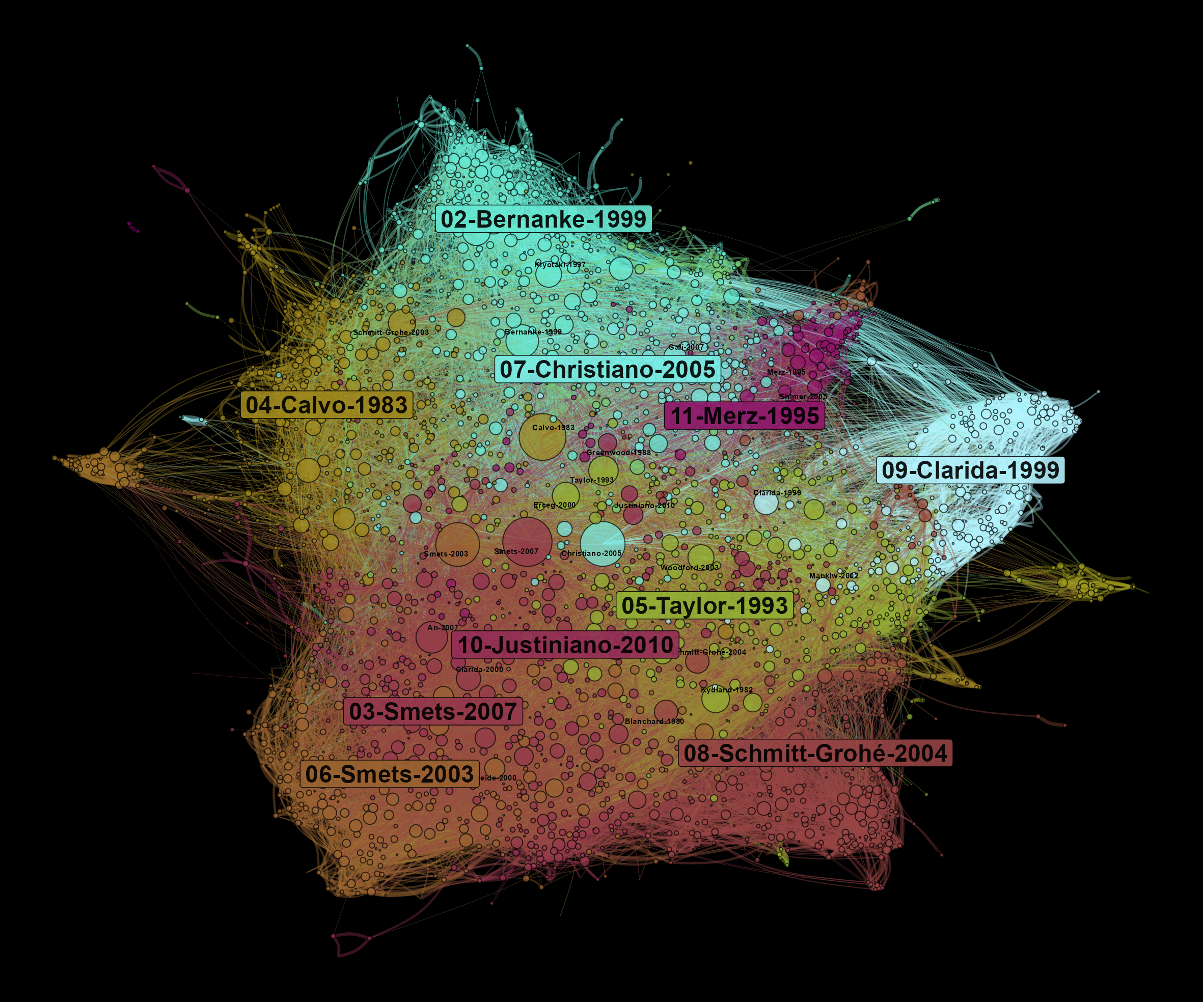
Figure 5: Bibliographic coupling network of articles using DSGE models
Let’s conclude by observing what are the most cited nodes in each community. We see that community 04 deals with international issues while the 07 is linked to fiscal policy issues.
ragg::agg_png(here("content", "en", "post", "2022-01-31-extracting-biblio-data-1", "top-ref-country-1.png"),
              width = 35,
              height = 30,
              units = "cm",
              res = 200)
top_nodes(graph,
          ordering_column = "size",
          top_n_per_com = 6,
          biggest_community = TRUE,
          community_threshold = 0.04) %>%
  select(Community_name, Label, title, n, color) %>%
  mutate(label = paste0(Label, "-", title) %>%
           str_wrap(34),
         label = tidytext::reorder_within(label, n, Community_name)) %>%
  ggplot(aes(n, label, fill = color)) +
  geom_col(show.legend = FALSE) +
  scale_fill_identity() +
  facet_wrap(~Community_name, ncol = 3, scales = "free") +
  tidytext::scale_y_reordered() +
  labs(x = "Number of citations", y = NULL) +
  theme_classic(base_size = 11)
invisible(dev.off())
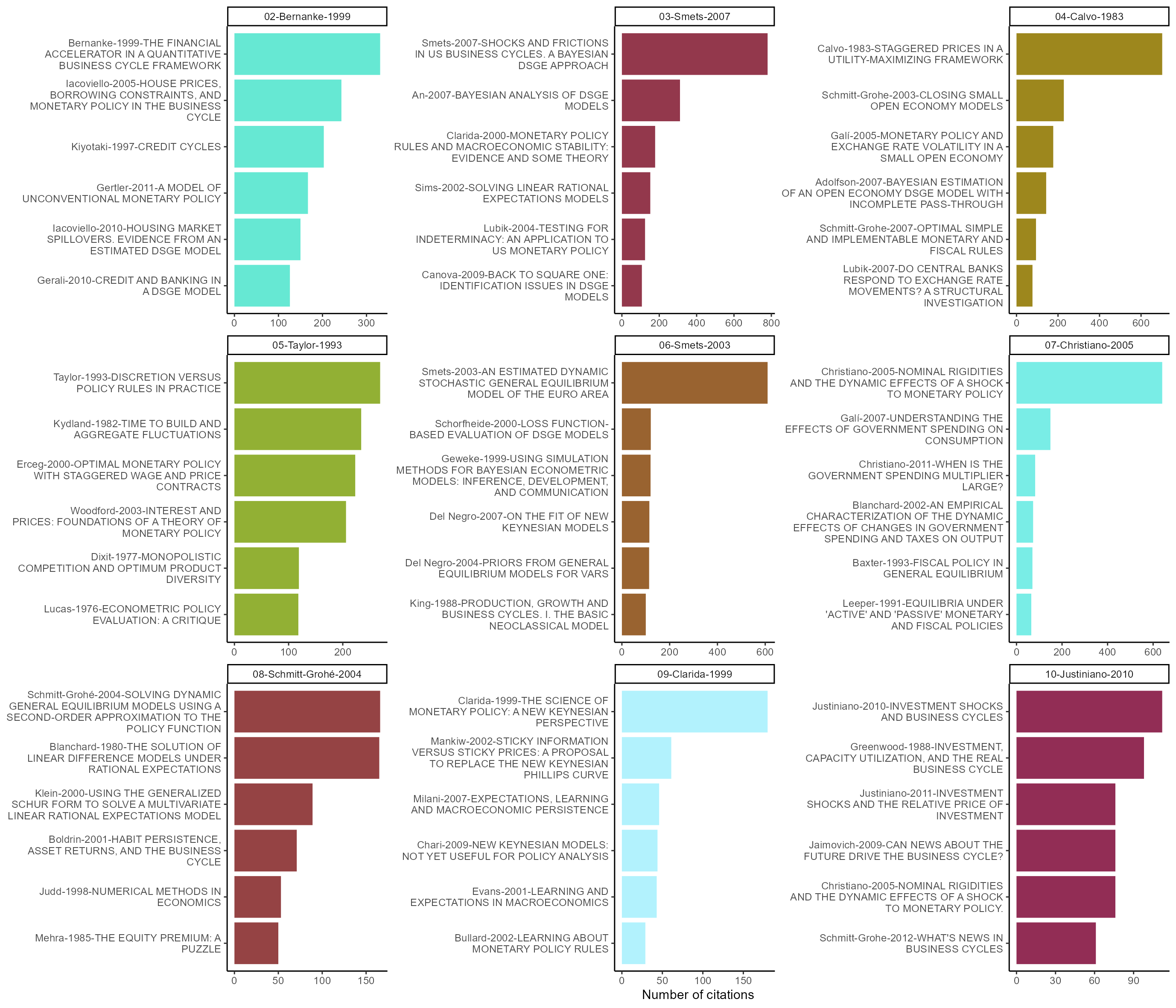
Figure 6: Most cited references per communities
References
Christiano, Lawrence J., Martin Eichenbaum, and Charles L. Evans. 2005. “Nominal Rigidities and the Dynamic Effects of a Shock to Monetary Policy.” Journal of Political Economy 113 (1): 1–45.
De Vroey, Michel. 2016. A History of Macroeconomics from Keynes to Lucas and Beyond. Cambridge: Cambridge University Press.
Goutsmedt, Aurélien, François Claveau, and Alexandre Truc. 2021. Biblionetwork: Create Different Types of Bibliometric Networks.
Kydland, Finn E., and Edward C. Prescott. 1982. “Time to Build and Aggregate Fluctuations.” Econometrica: Journal of the Econometric Society 50 (6): 1345–70.
Pedersen, Thomas Lin. 2020. Tidygraph: A Tidy API for Graph Manipulation. https://CRAN.R-project.org/package=tidygraph.
Sergi, Francesco. 2020. “The Standard Narrative about DSGE Models in Central Banks’ Technical Reports.” The European Journal of the History of Economic Thought 27 (2): 163–93.
Smets, Frank, and Raf Wouters. 2003. “An Estimated Dynamic Stochastic General Equilibrium Model of the Euro Area.” Journal of the European Economic Association 1 (5): 1123–75.
Smets, Frank, and Rafael Wouters. 2007. “Shocks and Frictions in US Business Cycles: A Bayesian DSGE Approach.” American Economic Review 97 (3): 586–606.
Vines, David, and Samuel Wills. 2018. “The Rebuilding Macroeconomic Theory Project: An Analytical Assessment.” Oxford Review of Economic Policy 34 (1-2): 1–42. https://doi.org/10.1093/oxrep/grx062.
Wickham, Hadley. 2021. Tidyverse: Easily Install and Load the Tidyverse. https://CRAN.R-project.org/package=tidyverse.
Wickham, Hadley, Mara Averick, Jennifer Bryan, Winston Chang, Lucy D’Agostino McGowan, Romain François, Garrett Grolemund, et al. 2019. “Welcome to the tidyverse.” Journal of Open Source Software 4 (43): 1686. https://doi.org/10.21105/joss.01686.
Don’t worry if you don’t understand regex at the beginning, that is a good occasion to learn and to practice. You can find simpler examples here and learn
stringrby the same occasion. ↩︎For reflexive and historical discussions of DSGE models, see De Vroey (2016, chap. 20), Vines and Wills (2018) and Sergi (2020). ↩︎
Normally, you won’t be able to download all the data in one extraction as there is a 2000 items limit, and thus you will need to do it in two steps. The easiest is to filter by year. ↩︎
We remove all
citationsdata.framesthat are empty (i.e. when an article cites nothing). ↩︎I will try to check that for another tutorial on bibliometric data, but I observed that I got fewer citations with the API method than with the Scopus website method. It means perhaps that if Scopus has not been able to give an identifier to a reference (perhaps because of not sufficiently clean metadata), the citation of this reference is removed from the data. Consequently, if our cleaning method is good, we could be able to keep more citations and thus to keep references that could be excluded in the APIs data extraction. ↩︎
I have perhaps forget some useful combinations. ↩︎
Most of the differences are due to the authors’ initials: some reference have only one when others have two initials for some authors. ↩︎
In case you want to know more on the different commands of anystyle, see the API documentation. ↩︎
As I find anystyle a very interesting tool, I will try to work on that issue in the following months and find a solution. An easy way to do it would perhaps be to save one
.txtper citing article and to run anystyle for all the.txt. We will have as many.bibas articles and we will just have to bind the resultingdata.frames. ↩︎
Aurélien Goutsmedt
Post-Doctoral Researcher
My research interests include history of economics, economic expertise and bibliometrics.