Extracting and Cleaning Bibliometric Data with R (2)
Exploring Dimensions
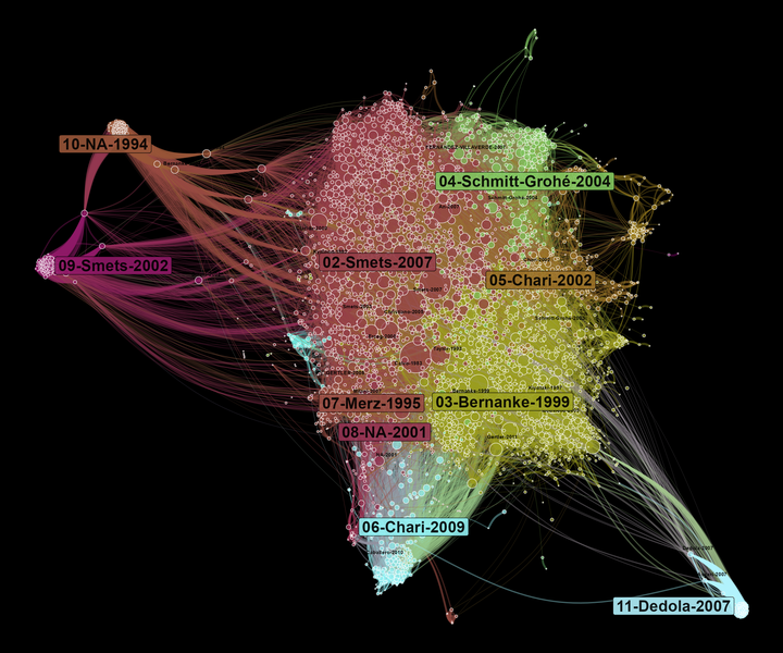
Table of Contents
The last post dealt with extracting bibliometric data from Scopus and presented some steps to clean these data, notably references data, with R. We will do something similar here, but for another database: Dimensions. Dimensions is a relatively newcomer in the world of bibliometric database, in comparison to Scopus or Web of Science. The initial advantage of Dimensions is that the search application is open to any one (if I remember well, you just have to create an account).1
Search on Dimensions website
So let’s begin with the same search than in the last post: publications using Dynamic Stochastic General Equilibrium model.2 Like with Scopus, we search for “DSGE” or “Dynamic Stochastic General Equilibrium”. A difference here is that we can choose between search in “full data” (meaning searching also in the full-text) or in “Title and abstract” (see Figure 1). Doing the first search, we get 27 693 results on February 4, 2022. The fact that we get close to 100 results before the 1990s (when the label DSGE began to be used) means that we could have a lot of false positive. It should be explored more in-depth. But for now and for this tutorial, we will opt for a more secure search, by focusing on titles and abstracts.
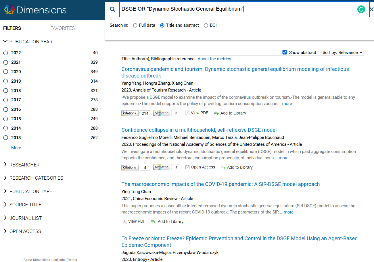
Figure 1: Our search on Dimensions app
We obtain 4106 results on February 4, 2022. That is quite much than the 2633 results of our Scopus search in the last post. But I think that it can be partly explain by the fact that Dimensions integrate “preprints” and we have 1532 preprints in our results.
To download the result, click on “Save / Export” on the right of the search bar, and then “Export results”. Two types of export are of interest for us: “Export full record” and “Export for bibliometric mapping”. In the first case, we can export only 500 results against 2500 for the second one (see Figure 2). This is not obvious, but the second option allows you to export most metadata, including affiliations and the references cited. What do we lose in comparison to the first export? The publication type (article, preprints, etc…), acknowledgements (that can be useful; see for instance Paul-Hus et al. 2017) and categorization of publications. That is not so much. Besides, it means that, by using the second option, you can extract more results than in Scopus (limited to 2000).
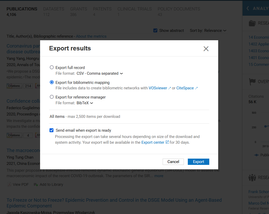
Figure 2: Choosing the export format
Another advantage of Dimensions over Scopus is that the data exported are quite easier to clean. So let’s load the needed packages and start the cleaning.
# packages
package_list <- c(
  "here", # use for paths creation
  "tidyverse",
  "janitor", # useful functions for cleaning imported data
  "biblionetwork", # creating edges
  "tidygraph", # for creating networks
  "ggraph" # plotting networks
)
for (p in package_list) {
  if (p %in% installed.packages() == FALSE) {
    install.packages(p, dependencies = TRUE)
  }
  library(p, character.only = TRUE)
}

github_list <- c(
  "agoutsmedt/networkflow", # manipulating network
  "ParkerICI/vite" # needed for the spatialisation of the network
)
for (p in github_list) {
  if (gsub(".*/", "", p) %in% installed.packages() == FALSE) {
    devtools::install_github(p)
  }
  library(gsub(".*/", "", p), character.only = TRUE)
}

# paths
data_path <- here(path.expand("~"),
                  "data",
                  "tuto_biblio_dsge")
dimensions_path <- here(data_path,
                    "dimensions")
Cleaning Dimensions data
Here are the data, extracted in two steps as we have more than 2500 items:
dimensions_data_1 <- read_csv(here(dimensions_path,
                                "dimensions_dsge_data_2015-2022.csv"),
                           skip = 1)
dimensions_data_2 <- read_csv(here(dimensions_path,
                                            "dimensions_dsge_data_1996-2014.csv"),
                                       skip = 1)

dimensions_data <- rbind(dimensions_data_1,
                                  dimensions_data_2) %>%
  clean_names() # cleaning column names with janitor to transform them

dimensions_data
## # A tibble: 4,097 x 15
##    publication_id doi      title abstract source_title_an~ pub_year volume issue
##    <chr>          <chr>    <chr> <chr>    <chr>               <dbl> <chr>  <chr>
##  1 pub.1126055399 10.1016~ Coro~ •We pro~ Annals of Touri~     2020 83     <NA>
##  2 pub.1143049966 10.1016~ The ~ This pa~ China Economic ~     2021 71     <NA>
##  3 pub.1126582656 10.1073~ Conf~ We inve~ Proceedings of ~     2020 117    17
##  4 pub.1133125128 10.3390~ To F~ The ong~ Entropy              2020 22     12
##  5 pub.1136926910 10.1002~ Impa~ Coronav~ Managerial and ~     2021 42     7
##  6 pub.1124254349 10.3390~ Macr~ Assessm~ Entropy              2020 22     2
##  7 pub.1120723604 10.1016~ Carb~ In rece~ The Science of ~     2019 697    <NA>
##  8 pub.1144700962 10.3390~ Immu~ The COV~ Entropy              2022 24     1
##  9 pub.1141415103 10.1016~ Ener~ Since t~ Structural Chan~     2021 59     <NA>
## 10 pub.1128536448 10.1177~ Does~ This ar~ Journal of Hosp~     2020 45     1
## # ... with 4,087 more rows, and 7 more variables: pagination <chr>,
## #   authors <chr>, authors_affiliations_name_of_research_organization <chr>,
## #   authors_affiliations_country_of_research_organization <chr>,
## #   dimensions_url <chr>, times_cited <dbl>, cited_references <chr>
We don’t need to give an ID to our documents as there is already a publications_id column.3
Cleaning duplicates
One issue with Dimensions is that it integrates preprints, which can be interesting for certain types of analysis.4 However, by using the “Export for bibliometric mapping” option (see the previous section), we cannot know if an item is a preprint or not. The consequence is that i) we can have duplicates (the same article with the preprint(s) and then the published version) but ii) we cannot discriminate between these duplicates as we don’t know which one is the published version. What we can do is to spot the duplicates thanks to the title and keep one of the duplicates depending on the presence of references or not.5 In other words, we keep the document for which we have references, and we do not care of which one we keep if all have references.6
duplicated_articles <- dimensions_data %>%
  add_count(title) %>%
  filter(n > 1) %>%
  arrange(title, cited_references)

to_keep <- duplicated_articles %>%
  group_by(title) %>%
  slice_head(n = 1)

to_remove <- duplicated_articles %>%
  filter(! publication_id %in% to_keep$publication_id)

dimensions_data <- dimensions_data %>%
  filter(! publication_id %in% to_remove$publication_id)
Cleaning affiliations
The goal now is to create a table which associates each document to authors’ affiliation (column authors_affiliations_name_of_research_organization) and the country of the affiliation (column authors_affiliations_country_of_research_organization). We cannot associate affiliations directly to authors as documents can have more authors than affiliations, and conversely.
dimensions_affiliations <- dimensions_data %>%
  select(publication_id,
         authors_affiliations_name_of_research_organization,
         authors_affiliations_country_of_research_organization) %>%
  separate_rows(starts_with("authors"), sep = "; ")

knitr::kable(head(dimensions_affiliations))
| publication_id | authors_affiliations_name_of_research_organization | authors_affiliations_country_of_research_organization |
|---|---|---|
| pub.1126055399 | Temple University | United States |
| pub.1126055399 | Jiangxi University of Finance and Economics | China |
| pub.1126055399 | University of Connecticut | United States |
| pub.1143049966 | Beijing Normal University | China |
| pub.1126582656 | Laboratory of Theoretical Physics of Condensed Matter | France |
| pub.1126582656 | École Polytechnique | France |
We can now compare the country of affiliations for the dimensions document and for the Scopus affiliation cleaned in the previous post. We first bind together affiliations of DSGE articles from Scopus and Dimensions.
scopus_affiliations <- read_rds(here(data_path,
                                     "scopus",
                                     "data_cleaned",
                                     "scopus_affiliations.rds")) %>%
  mutate(data = "scopus") %>%
  select(-authors)

dimensions_affiliations <- dimensions_affiliations %>%
  mutate(data = "dimensions")

affiliations <- dimensions_affiliations %>%
  rename("affiliations" = authors_affiliations_name_of_research_organization,
         "country" = authors_affiliations_country_of_research_organization,
         "citing_id" = publication_id) %>%
  bind_rows(scopus_affiliations)
In Figure @ref(fig:country_affiliations), we can observe that the ranking is almost the same at least for the first 8 countries. Nonetheless, while we have more documents in Dimensions(3856) than in Scopus (2565), we have a relatively equivalent number of affiliations in both corpus: 5502 for Dimensions against 5461 for Scopus. Besides, we count more NA values (1132) than affiliations from United States (1112) in Dimensions, meaning that a lot of information is missing.
affiliations %>%
  filter(!is.na(country)) %>%
  group_by(data) %>%
  count(country) %>%
  mutate(proportion = n/sum(n)) %>%
  slice_max(order_by = proportion, n = 10, with_ties = FALSE) %>%
  mutate(country = tidytext::reorder_within(country, proportion, data)) %>% # see https://juliasilge.com/blog/reorder-within/ for more info
  ggplot(aes(proportion, country, fill = data)) +
  geom_col(show.legend = FALSE) +
  facet_wrap(~data, scales = "free_y") +
  tidytext::scale_y_reordered() +
  labs(x = "Proportion of the Country in all affiliations (excluding NA)") +
  theme_classic(base_size = 16)
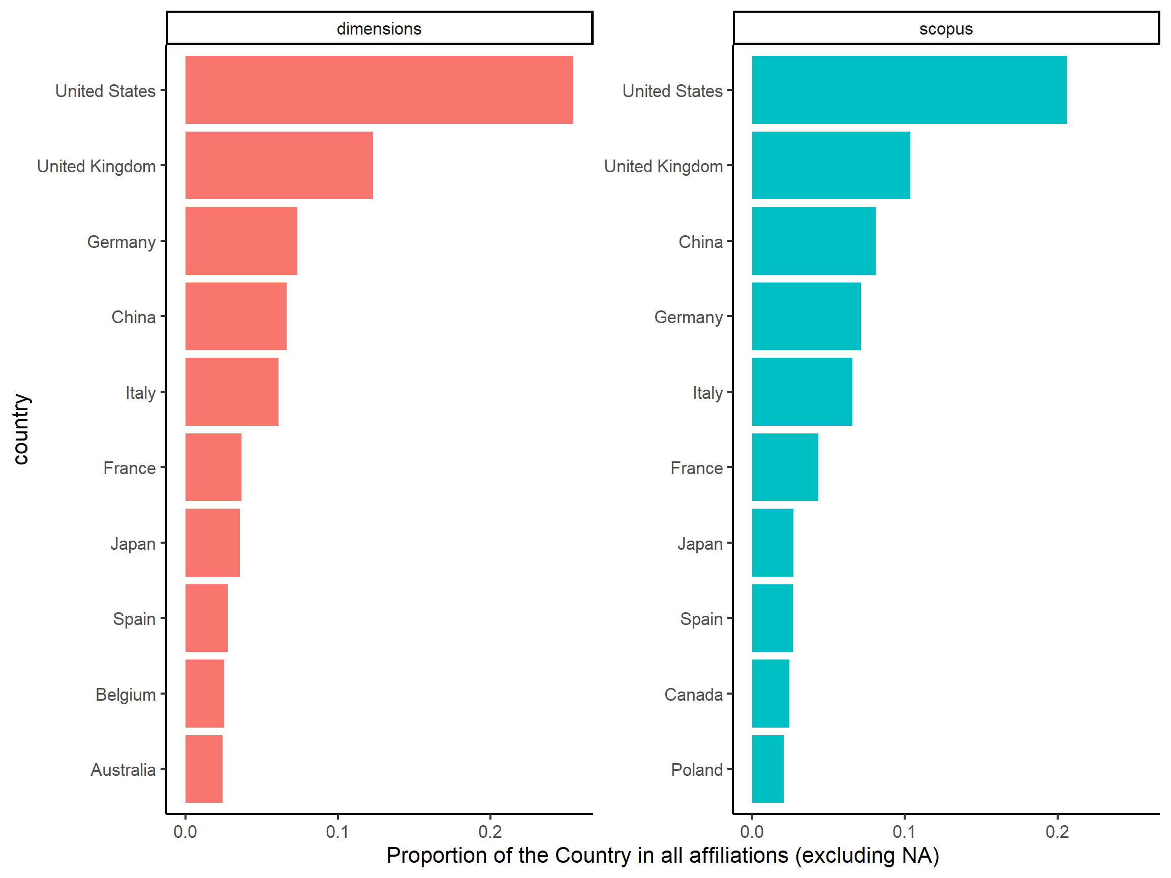
Figure 3: Top countries for affiliations in Scopus and Dimensions
Cleaning references
Cleaning the references is quite easy for Dimensions:
- you have a clear separator between the references of each citing document: a semi-colon before a square bracket;
- you have the same information for each references (see
column_names) even if the information is lacking, and you have a simple separator between information:|.
references_extract <- dimensions_data %>%
  filter(! is.na(cited_references)) %>%
  rename("citing_id" = publication_id) %>% # because the "publication_id" column is also the identifier of the reference
  select(citing_id, cited_references) %>%
  separate_rows(cited_references, sep = ";(?=\\[)") %>%
  as_tibble

column_names <- c("authors",
                  "author_id",
                  "source",
                  "year",
                  "volume",
                  "issue",
                  "pagination",
                  "doi",
                  "publication_id",
                  "times_cited")

dimensions_direct_citation <- references_extract %>%
  separate(col = cited_references, into = column_names, sep = "\\|")

knitr::kable(head(dimensions_direct_citation, n = 5))
| citing_id | authors | author_id | source | year | volume | issue | pagination | doi | publication_id | times_cited |
|---|---|---|---|---|---|---|---|---|---|---|
| pub.1126055399 | [Yagihashi, Takeshi; Du, Juan] | [ur.07662443654.76; ur.013363010625.14] | Economic Inquiry | 2015 | 53 | 3 | 1556-1579 | 10.1111/ecin.12204 | pub.1003172294 | 5 |
| pub.1126055399 | [Yan, Qi; Zhang, Hanqin Qiu] | [; ] | Asia Pacific Journal of Tourism Research | 2012 | 17 | 5 | 534-550 | 10.1080/10941665.2011.627929 | pub.1052463830 | 5 |
| pub.1126055399 | [Barro, Robert J] | [] | The Quarterly Journal of Economics | 2006 | 121 | 3 | 823-866 | 10.1162/qjec.121.3.823 | pub.1063352797 | 1133 |
| pub.1126055399 | [Hall, R. E.; Jones, C. I.] | [; ] | The Quarterly Journal of Economics | 2007 | 122 | 1 | 39-72 | 10.1162/qjec.122.1.39 | pub.1063352822 | 450 |
| pub.1126055399 | [Gourio, François] | [] | American Economic Review | 2012 | 102 | 6 | 2734-2766 | 10.1257/aer.102.6.2734 | pub.1064525837 | 372 |
Another advantage is that, as for Scopus API (but not for data extracted on Scopus website), references already have an identifier.7 It means that you don’t have to match the citations together to find which documents are citing the same references (what we had to do here). Thus, you can easily extract the list of the distinct references cited in your corpus, and it will make easier the building of a co-citation network later.
dimensions_references <- dimensions_direct_citation %>%
  distinct(publication_id, .keep_all = TRUE) %>%
  select(-citing_id)

knitr::kable(tail(dimensions_references, n = 5))
| authors | author_id | source | year | volume | issue | pagination | doi | publication_id | times_cited |
|---|---|---|---|---|---|---|---|---|---|
| [Barro, Robert J.; Grossman, Herschel I.] | [ur.01313542524.54; ur.015506435407.81] | The Review of Economic Studies | 1974 | 41 | 1 | 87 | 10.2307/2296401 | pub.1069867975 | 65 |
| [Benassy, Jean-Pascal] | [] | Scandinavian Journal of Economics | 1977 | 79 | 2 | 147 | 10.2307/3439505 | pub.1070324476 | 41 |
| [Delli Gatti, Domenico; Gallegati, Marco; Minsky, Hyman P.] | [ur.011273107226.57; ; ur.015265626417.37] | SSRN Electronic Journal | 1998 | 10.2139/ssrn.125848 | pub.1102184434 | 20 | |||
| [Beker, Victor A.] | [] | SSRN Electronic Journal | 2005 | 10.2139/ssrn.839307 | pub.1102214017 | 5 | |||
| [Beker, Victor A.] | [] | SSRN Electronic Journal | 2010 | 10.2139/ssrn.1730222 | pub.1102299065 | 7 |
However, there is one problem with Dimensions ID: I suppose that Dimensions is able to match references together thanks to DOI that are often present in references data (more than in Scopus references data). The problem is that some references (in general books and chapters in books) lack many (actually almost all) information, like authors and publishing source. It means that we are not able to know what it is, if not by entering the DOI in a web browser. We will encounter this problem again when building the network.
As for affiliations country, we can compare the most cited references in Dimensions and in Scopus. We first extract the top 10 for Scopus and Dimensions:
scopus_direct_citation <- read_rds(here(data_path,
                                        "scopus",
                                        "data_cleaned",
                                        "scopus_manual_direct_citation.rds"))
scopus_references <- read_rds(here(data_path,
                                   "scopus",
                                   "data_cleaned",
                                   "scopus_manual_references.rds"))

scopus_top_ref <- scopus_direct_citation %>%
  add_count(new_id_ref) %>%
  mutate(proportion = n/n()) %>%
  select(new_id_ref, proportion) %>%
  unique() %>%
  slice_max(proportion, n = 10) %>%
  left_join(select(scopus_references, new_id_ref, references)) %>%
  select(references, proportion) %>%
  mutate(data = "scopus",
         references = str_extract(references, ".*\\(\\d{4}\\)")) # cleaning for plotting

dimensions_references <- dimensions_references %>%
  mutate(references = paste0(authors, ", ", year, ", ", source))

dimensions_top_ref <- dimensions_direct_citation %>%
  add_count(publication_id) %>%
  mutate(proportion = n/n()) %>%
  select(publication_id, proportion) %>%
  unique() %>%
  slice_max(proportion, n = 10) %>%
  left_join(select(dimensions_references, publication_id, references)) %>%
  select(references, proportion) %>%
  mutate(data = "dimensions")
We can see in Figure 4 that the 10 most cited references are the same, only the ranking is changing after the fourth position
dimensions_top_ref %>%
  bind_rows(scopus_top_ref) %>%
  mutate(references = str_wrap(references, 35)) %>%
  ggplot(aes(proportion, fct_reorder(references, proportion), fill = data)) +
  geom_col(show.legend = FALSE) +
  facet_wrap(~data, scales = "free") +
  tidytext::scale_y_reordered() +
  labs(x = "Proportion on all citations") +
  theme_classic(base_size = 13)
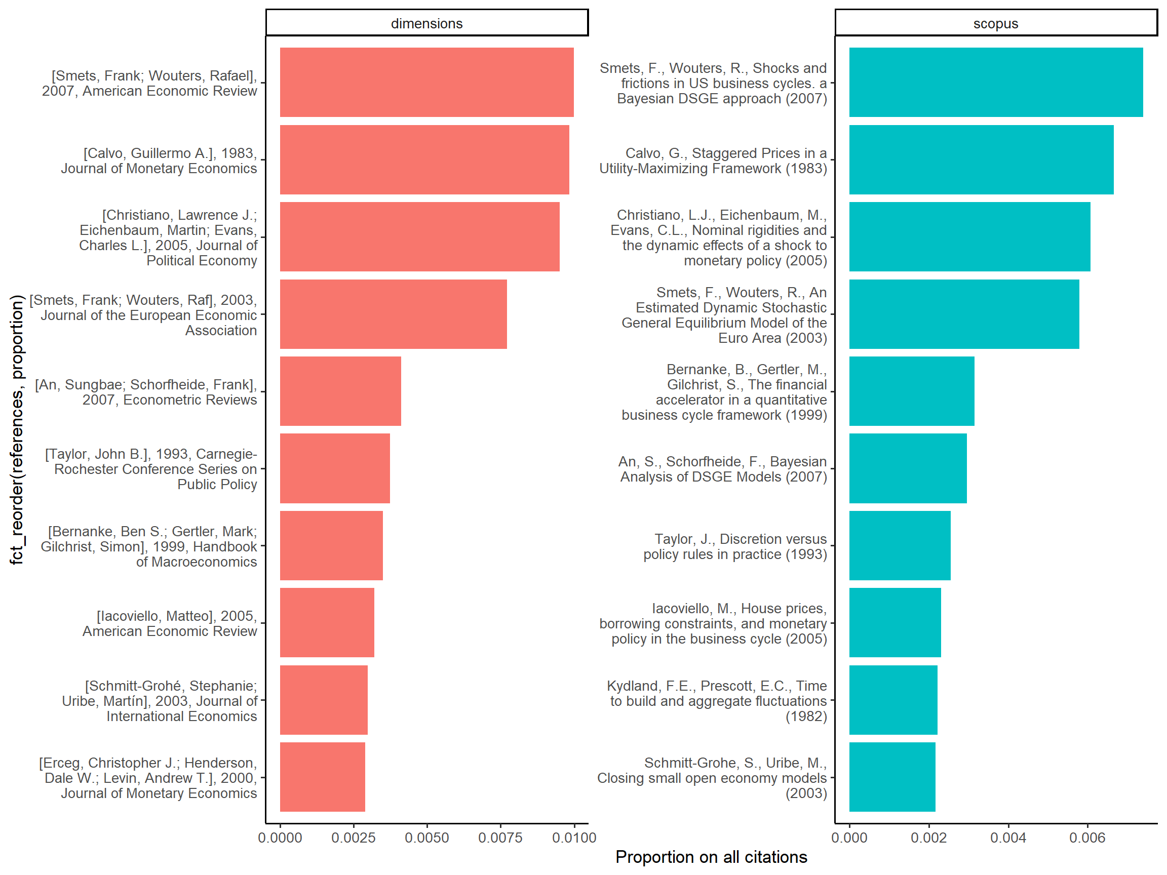
Figure 4: Top references of DSGE documents in Scopus and Dimensions
Building co-citation network
Here, we follow what we have done for Scopus here. We use the biblio_cocitation function of the biblionetwork package to build the list of edges between our nodes (i.e. the references). The edge between two nodes is weighted depending of the total number of times each reference has been cited in the whole Dimensions DSGE corpus (see here for more details).
citations <- dimensions_direct_citation %>%
  add_count(publication_id) %>%
  select(publication_id, n) %>%
  unique

references_filtered <- dimensions_references %>%
  left_join(citations) %>%
  filter(n >= 5)

edges <- biblionetwork::biblio_cocitation(filter(dimensions_direct_citation, publication_id %in% references_filtered$publication_id),
                                          "citing_id",
                                          "publication_id",
                                          weight_threshold = 3)
edges
##                  from             to     weight         Source         Target
##     1: pub.1000001876 pub.1008725945 0.18814417 pub.1000001876 pub.1008725945
##     2: pub.1000001876 pub.1008947877 0.03468730 pub.1000001876 pub.1008947877
##     3: pub.1000001876 pub.1013813490 0.07749843 pub.1000001876 pub.1013813490
##     4: pub.1000001876 pub.1050095878 0.14301939 pub.1000001876 pub.1050095878
##     5: pub.1000001876 pub.1064524465 0.06073322 pub.1000001876 pub.1064524465
##    ---
## 71877: pub.1119779752 pub.1125952654 0.40824829 pub.1119779752 pub.1125952654
## 71878: pub.1134024220 pub.1135197325 0.10846523 pub.1134024220 pub.1135197325
## 71879: pub.1134024220 pub.1135197780 0.16888013 pub.1134024220 pub.1135197780
## 71880: pub.1142606957 pub.1142611529 0.13155870 pub.1142606957 pub.1142611529
## 71881: pub.1142606957 pub.1143248862 0.10241831 pub.1142606957 pub.1143248862
We can now create a graph using tidygraph (Pedersen 2020) and networkflow.8
references_filtered <- references_filtered %>%
  relocate(publication_id, .before = authors) # first column has to be the identifier

graph <- tbl_main_component(nodes = references_filtered,
                            edges = edges,
                            directed = FALSE)
graph
## # A tbl_graph: 3561 nodes and 71876 edges
## #
## # An undirected simple graph with 1 component
## #
## # Node Data: 3,561 x 12 (active)
##   Id    authors author_id source year  volume issue pagination doi   times_cited
##   <chr> <chr>   <chr>     <chr>  <chr> <chr>  <chr> <chr>      <chr> <chr>
## 1 pub.~ [Barro~ []        The Q~ 2006  121    "3"   823-866    10.1~ 1133
## 2 pub.~ [Gouri~ []        Ameri~ 2012  102    "6"   2734-2766  10.1~ 372
## 3 pub.~ [Isoré~ [ur.0161~ Journ~ 2017  79     ""    97-125     10.1~ 27
## 4 pub.~ [Calvo~ [ur.0744~ Journ~ 1983  12     "3"   383-398    10.1~ 4413
## 5 pub.~ [Chris~ [ur.0114~ Handb~ 2010  3      ""    285-367    10.1~ 126
## 6 pub.~ [Heute~ [ur.0161~ Revie~ 2012  15     "2"   244-264    10.1~ 161
## # ... with 3,555 more rows, and 2 more variables: references <chr>, n <int>
## #
## # Edge Data: 71,876 x 5
##    from    to weight Source         Target
##   <int> <int>  <dbl> <chr>          <chr>
## 1    33   867 0.188  pub.1000001876 pub.1008725945
## 2     4   867 0.0347 pub.1000001876 pub.1008947877
## 3    12   867 0.0775 pub.1000001876 pub.1013813490
## # ... with 71,873 more rows
set.seed(1234)
graph <- leiden_workflow(graph) # identifying clusters of nodes

nb_communities <- graph %>%
  activate(nodes) %>%
  as_tibble %>%
  select(Com_ID) %>%
  unique %>%
  nrow
palette <- scico::scico(n = nb_communities, palette = "hawaii") %>% # creating a color palette
    sample()

graph <- community_colors(graph, palette, community_column = "Com_ID")

graph <- graph %>%
  activate(nodes) %>%
  mutate(size = n,# will be used for size of nodes
         first_author = str_extract(authors, "(?<=\\[)(.+?)(?=,)"),
         label = paste0(first_author, "-", year))

graph <- community_names(graph,
                         ordering_column = "size",
                         naming = "label",
                         community_column = "Com_ID")

graph <- vite::complete_forceatlas2(graph,
                                    first.iter = 10000)


top_nodes  <- top_nodes(graph,
                        ordering_column = "size",
                        top_n = 15,
                        top_n_per_com = 2,
                        biggest_community = TRUE,
                        community_threshold = 0.02)
community_labels <- community_labels(graph,
                                     community_name_column = "Community_name",
                                     community_size_column = "Size_com",
                                     biggest_community = TRUE,
                                     community_threshold = 0.02)
A co-citation network allows us to observe what are the main influences of a field of research. At the centre of the network, we find the most cited references. On the borders of the graph, there are specific communities that influence different parts of the literature on DSGE. Here, the size of nodes depends on the number of times they are cited in our corpus.
If we compare to the Scopus co-citation network, we find some similarities as the domination of the Smets and Wouters (2007) community.9 However, the network is less dense here and displays more marginal communities. The “NA-1994” community is a good example of what I was talking about above on Dimensions identifying process. “NA-1994” (the biggest node of this community) is actually Hamilton (1994).
graph <- graph %>%
  activate(edges) %>%
  filter(weight > 0.05)

ggraph(graph, "manual", x = x, y = y) +
  geom_edge_arc0(aes(color = color_edges, width = weight), alpha = 0.4, strength = 0.2, show.legend = FALSE) +
  scale_edge_width_continuous(range = c(0.1,2)) +
  scale_edge_colour_identity() +
  geom_node_point(aes(x=x, y=y, size = size, fill = color), pch = 21, alpha = 0.7, show.legend = FALSE) +
  scale_size_continuous(range = c(0.3,16)) +
  scale_fill_identity() +
  ggnewscale::new_scale("size") +
  ggrepel::geom_text_repel(data = top_nodes, aes(x=x, y=y, label = Label), size = 2, fontface="bold", alpha = 1, point.padding=NA, show.legend = FALSE) +
  ggrepel::geom_label_repel(data = community_labels, aes(x=x, y=y, label = Community_name, fill = color), size = 6, fontface="bold", alpha = 0.9, point.padding=NA, show.legend = FALSE) +
  scale_size_continuous(range = c(0.5,5)) +
  theme_void()

Figure 5: Bibliographic coupling network of articles using DSGE models
The differences between Scopus and Dimensions co-citation network would deserve a more thorough investigation, which is outside the scope of this tutorial.10 So let’s conclude just by observing what are the most cited nodes in each community. Here, we can see more clearly that community 02 with represent to a certain extent the “core” of the literature at the basis of DSGE models. Community 04 deals more with econometric problems, while community 05 tackles international issues.
ragg::agg_png(here("content", "en", "post", "2022-02-03-extracting-biblio-data-2", "top_ref.png"),
              width = 30,
              height = 25,
              units = "cm",
              res = 200)
top_nodes(graph,
          ordering_column = "size",
          top_n = 10,
          top_n_per_com = 6,
          biggest_community = TRUE,
          community_threshold = 0.03) %>%
  select(Community_name, references, n, color) %>%
  mutate(label = str_wrap(references, 35),
         label = tidytext::reorder_within(label, n, Community_name)) %>%
  ggplot(aes(n, label, fill = color)) +
  geom_col(show.legend = FALSE) +
  scale_fill_identity() +
  facet_wrap(~Community_name, ncol = 3, scales = "free") +
  tidytext::scale_y_reordered() +
  labs(x = "Number of citations", y = NULL) +
  theme_classic(base_size = 10)
invisible(dev.off())
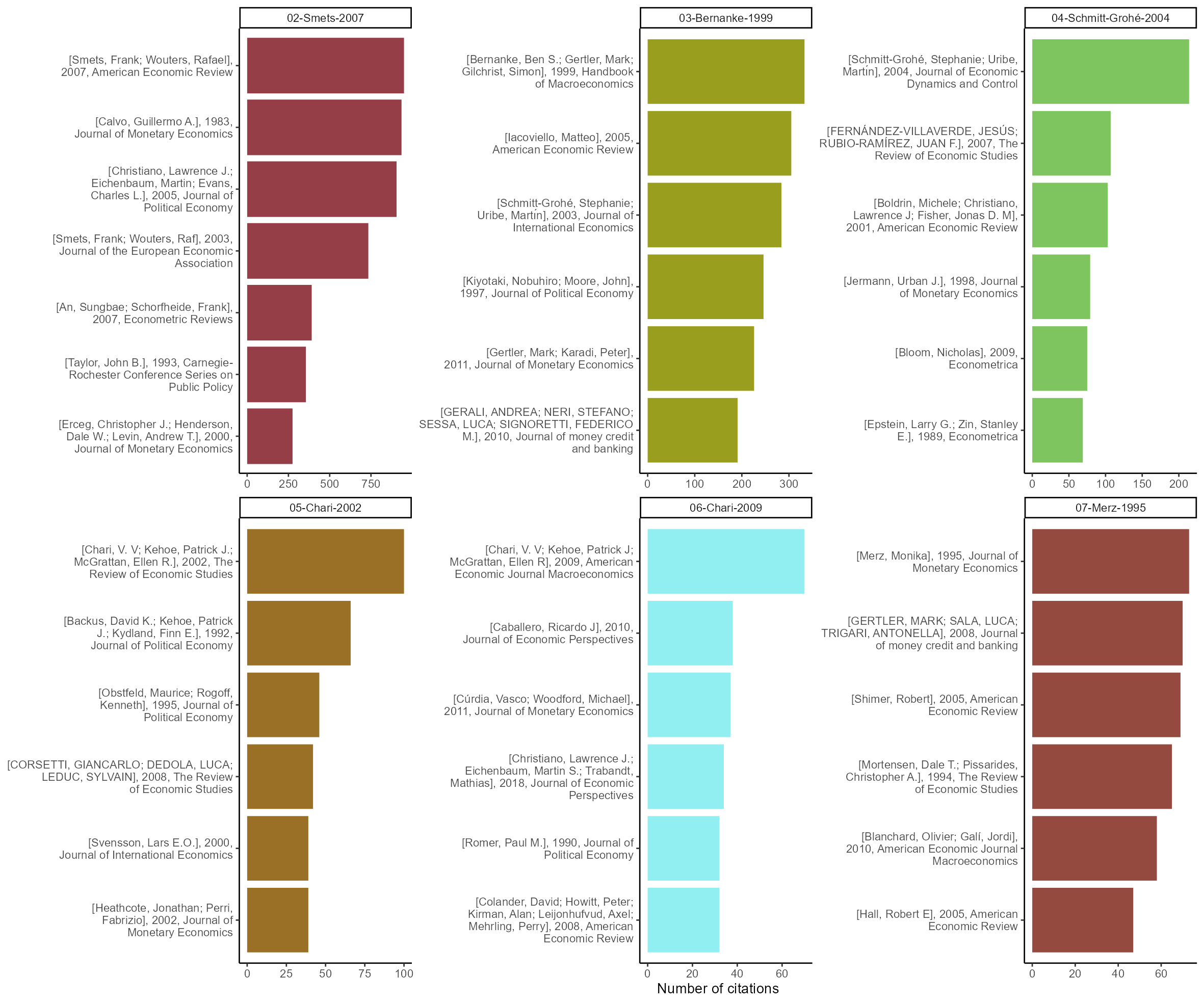
Figure 6: Most cited references per communities
References
Hamilton, James Douglas. 1994. Time Series Analysis. First. Princeton, N.J: Princeton University Press.
Paul-Hus, Adèle, Philippe Mongeon, Maxime Sainte-Marie, and Vincent Larivière. 2017. “The Sum of It All: Revealing Collaboration Patterns by Combining Authorship and Acknowledgements.” Journal of Informetrics 11 (1): 80–87. https://doi.org/10.1016/j.joi.2016.11.005.
Pedersen, Thomas Lin. 2020. Tidygraph: A Tidy API for Graph Manipulation. https://CRAN.R-project.org/package=tidygraph.
Smets, Frank, and Rafael Wouters. 2007. “Shocks and Frictions in US Business Cycles: A Bayesian DSGE Approach.” American Economic Review 97 (3): 586–606.
It exists also an API for which you can ask access. It would allow you to use the rdimensions package to query data. ↩︎
Keeping the same search allows us to do some comparisons with Scopus data and observe how it impacts networks and other results. ↩︎
A good practice is to clean and standardise column names by using the great
janitorpackage. By default,clean_names()use snake case names. ↩︎For instance, by studying what is eventually published and after how much time. ↩︎
It remains the possibility of “hidden” duplicates if the title have changed when the document has been published. ↩︎
Obviously, that is not the optimal method if what you want is to keep the published version. Here, you would need to exclude the preprints of the duplicates, for instance by removing items which display “SSRN” as their
source_title_anthology_title. Another option, if you don’t want preprints at all is just to uncheck preprints on Dimensions search application when you are extracting your data. ↩︎Be careful: the column is also called
publication_id, meaning that you have to change the name of the column with the identifier of citing articles. ↩︎I don’t enter in the details here as that is not the purpose of this tutorial and that the different steps are explained on
networkflowwebsite. ↩︎However, we can observe that if this community is still the biggest, it is bigger than in Scopus network and include more central references. ↩︎
Part of the differences comes from differences in the initial corpus and thus is linked to the difference in Scopus and Dimensions data (notably the journals that are integrated in the databases). Another part of the differences results from our own treatment of the data: a different cleaning of references, different thresholds used to select the nodes (as we use an absolute threshold, not a relative one), different types of documents (preprints and “hidden” duplicates), etc… ↩︎
Aurélien Goutsmedt
Post-Doctoral Researcher
My research interests include history of economics, economic expertise and bibliometrics.